Mapping Plant Observation Patterns Around Falcon Sightings
An exploratory spatial analysis combining iNaturalist observations, Python data preparation, QGIS, and R visualizations to examine how recorded plant taxa are distributed around falcon observation locations in the Ithaca, New York region.
Using spatial data to ask ecological questions
This project explores whether the plant taxa represented in iNaturalist observations near falcon observation locations differ from those recorded near randomly generated comparison locations. It combines community-contributed biodiversity records with spatial analysis in QGIS and descriptive visualizations in R.
The workflow brings together data acquisition, spatial processing, taxonomic summaries, and map-based communication. Falcon observation locations were buffered and compared with an equal number of random locations within a defined Ithaca-area study boundary. Plant observation records intersecting those sampling areas were then summarized and compared.
Research question & objectives
Are certain plant taxa disproportionately represented in iNaturalist observations surrounding falcon observation locations compared with randomly selected locations in the Ithaca study area?
Here, “represented” refers to the frequency and relative frequency of recorded plant observations. It does not imply that a plant is ecologically preferred by falcons or more abundant in the landscape.
01 · Characterize
Map and summarize plant observation records spatially associated with falcon buffers.
02 · Compare
Create a random-location comparison group within the same study boundary and summarize its associated plant records.
03 · Evaluate
Use descriptive statistics and visual comparisons to examine taxonomic representation, observation quality, and spatial structure.
04 · Improve
Identify how GIS methods, data quality, and sampling design can be strengthened for future biodiversity research.
Study area and sampling locations
The study-area polygon covers approximately 359.35 km² in the Ithaca, New York region. It defines the geographic extent for the falcon observations and the generation of random comparison locations. Both sampling groups contain 124 locations.
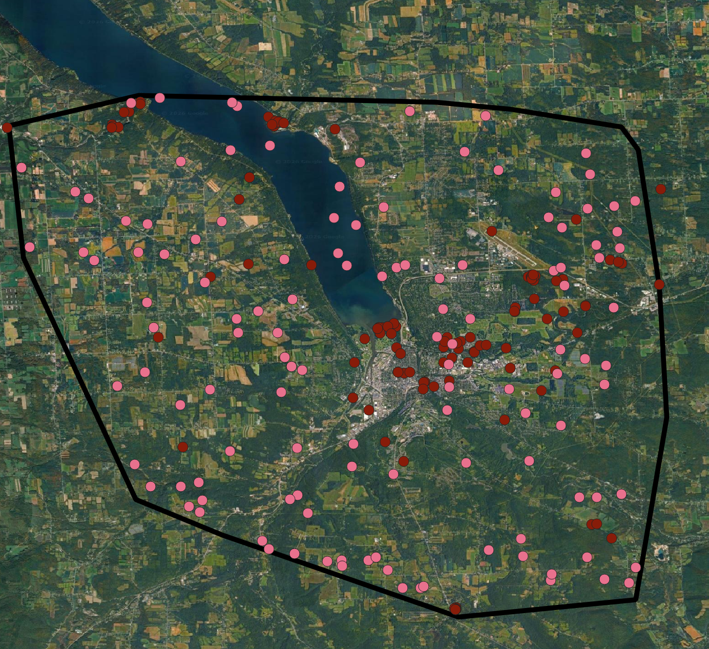
GIS workflow
The workflow combines point observations, polygon buffers, spatial selection, and taxonomic summaries. iNaturalist records were collected and prepared as georeferenced observation datasets, then organized and analyzed in QGIS and R.
Collect falcon observations
Compile 124 falcon observation locations within the study boundary. The records include observation identifiers, taxonomic names, dates, quality classifications, and coordinates.
Collect plant observations
Retrieve georeferenced plant records from iNaturalist, retaining taxonomic labels, observation identifiers, dates, quality classifications, and coordinates.
Create falcon-associated buffers
Create a buffer around each falcon location. The preliminary QGIS workflow used EPSG:4326 (WGS 84) and an entered distance of approximately 0.0009 degrees, intended to approximate 100 meters.
Generate random comparison locations
Generate 124 random points within the study-area polygon and create a corresponding set of buffers using the same approximate angular distance.
Associate plant observations spatially
Use spatial relationships in QGIS to identify plant records falling within the falcon-associated and random buffer areas.
Summarize and visualize
Create individual-observation and summary outputs, compare taxonomic-label frequencies and observation quality, and produce maps and charts in QGIS and R.
Data organization
| Dataset | Role in analysis | Current count |
|---|---|---|
| Falcon observation locations | Locations of recorded falcon sightings | 124 |
| Random comparison locations | Comparison locations within study boundary | 124 |
| Falcon buffers | Approximate areas around falcon observations | 124 polygons |
| Random buffers | Approximate areas around random locations | 124 polygons |
| Plants near falcons | Individual plant records spatially associated with falcon buffers | 426 records |
| Plants near random locations | Individual plant records spatially associated with random buffers | 46 records |
Preliminary findings
The current individual-observation layers contain more plant records associated with falcon buffers than with random buffers. The difference is descriptive: equal numbers of sampling locations do not guarantee equal observation effort, and the two groups differ in spatial clustering and total recorded observations.
| Measure | Falcon-associated | Random comparison |
|---|---|---|
| Sampling locations / buffers | 124 | 124 |
| Individual plant observation records | 426 | 46 |
| Distinct taxonomic labels in frequency output | 259 | 41 |
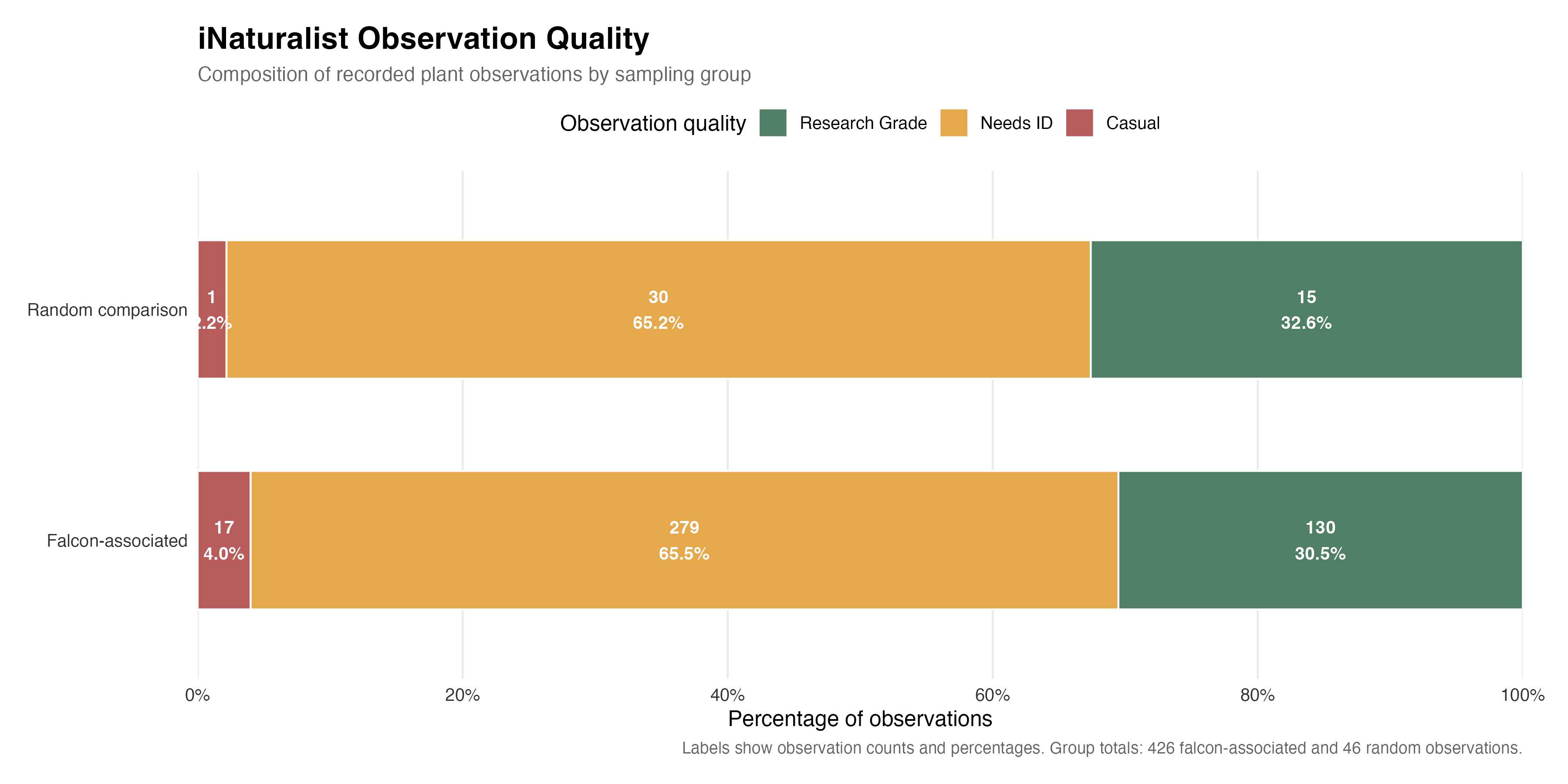
| Research Grade records | 130 (30.5%) | 15 (32.6%) |
| Needs ID records | 279 (65.5%) | 30 (65.2%) |
| Casual records | 17 (4.0%) | 1 (2.2%) |
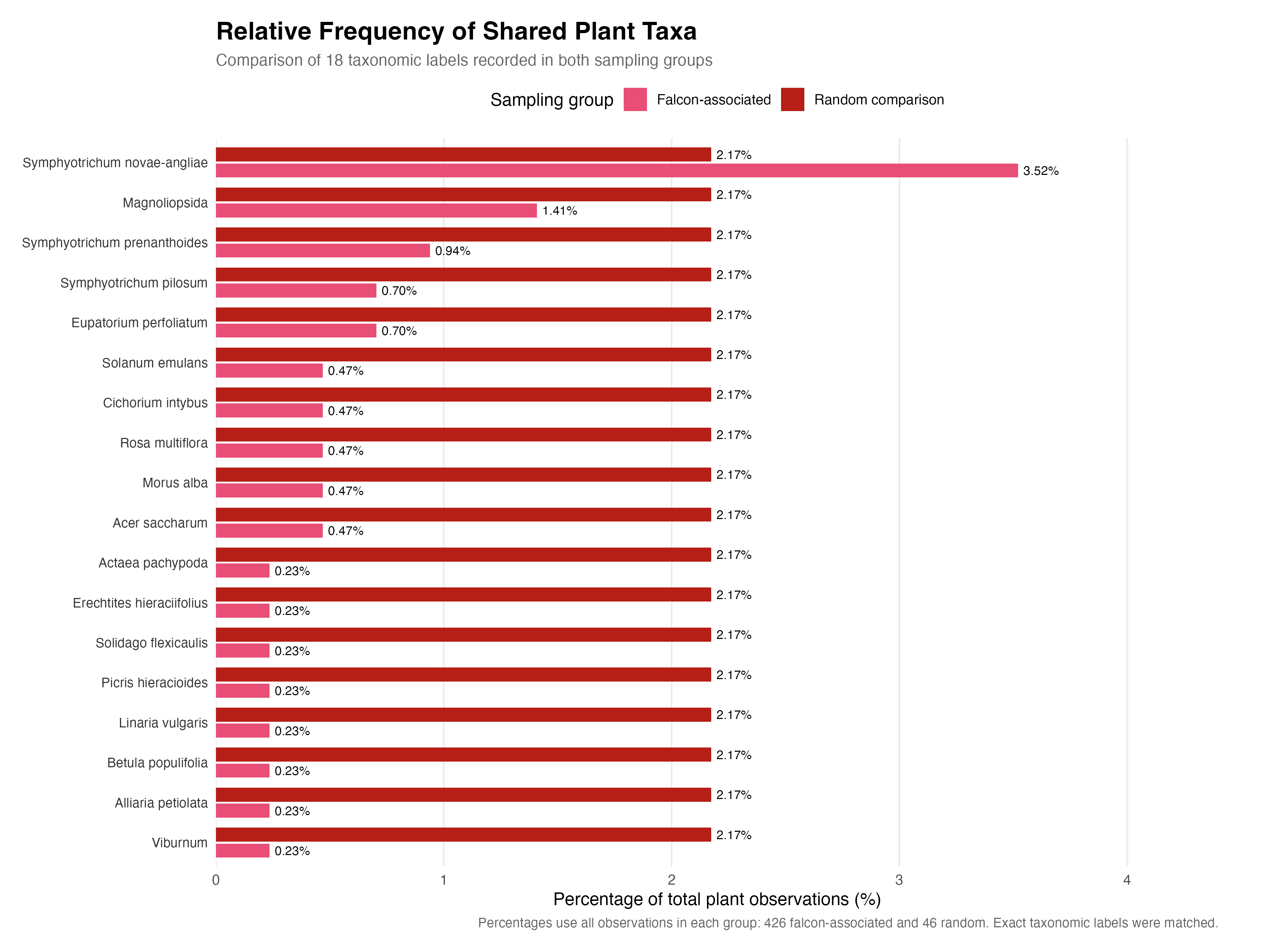
| Shared exact taxonomic labels | 18 | |
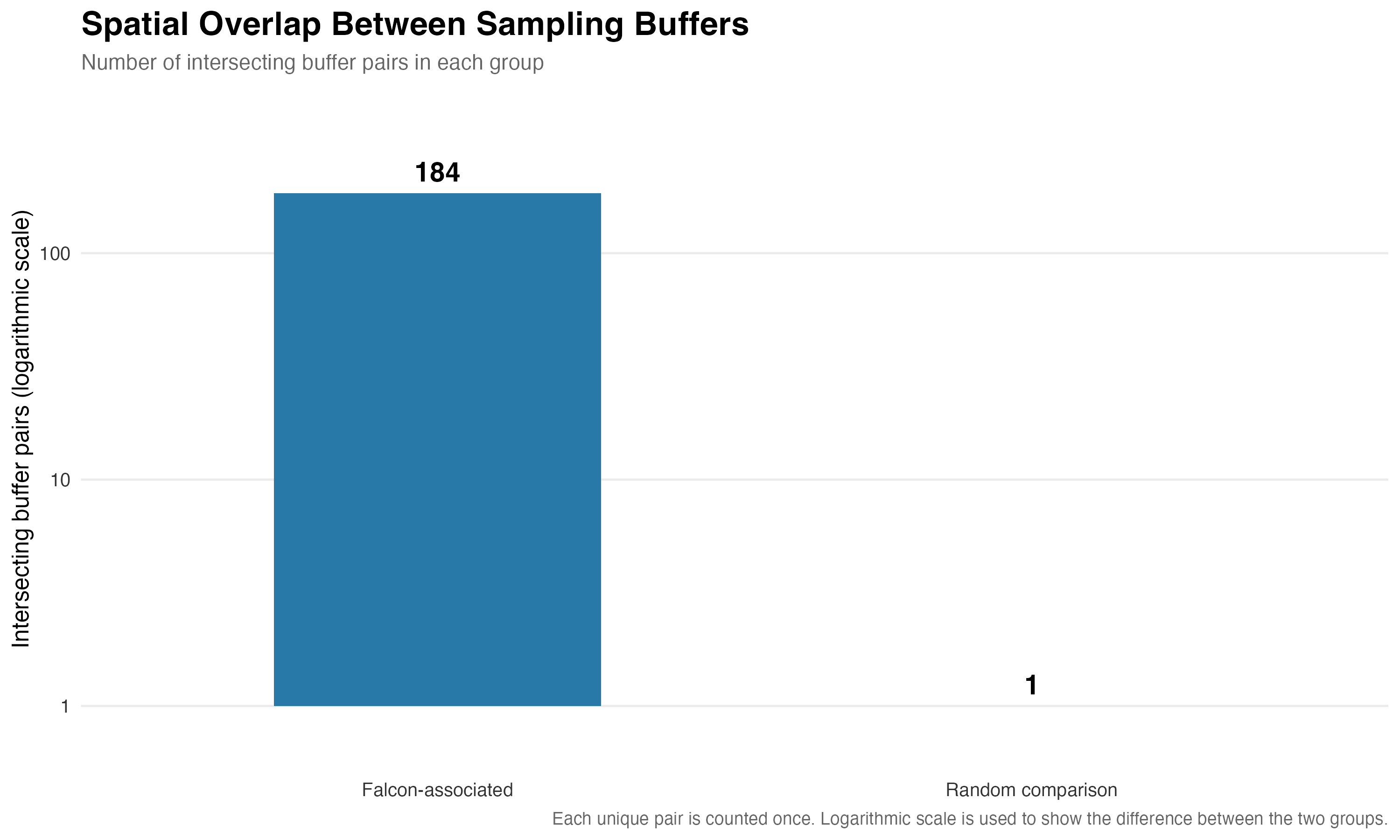
| Intersecting buffer pairs | 184 | 1 |
Frequently recorded taxonomic labels
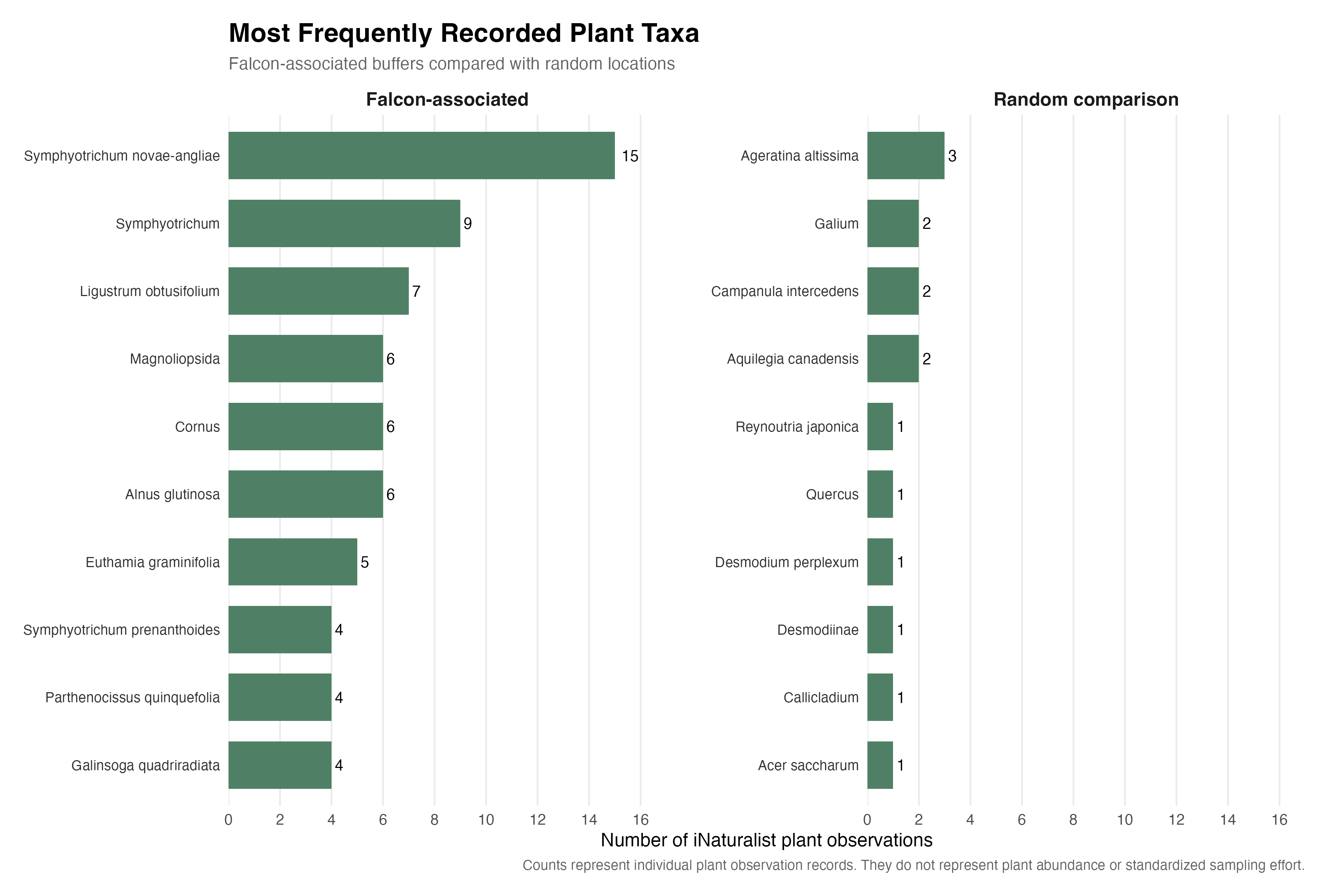
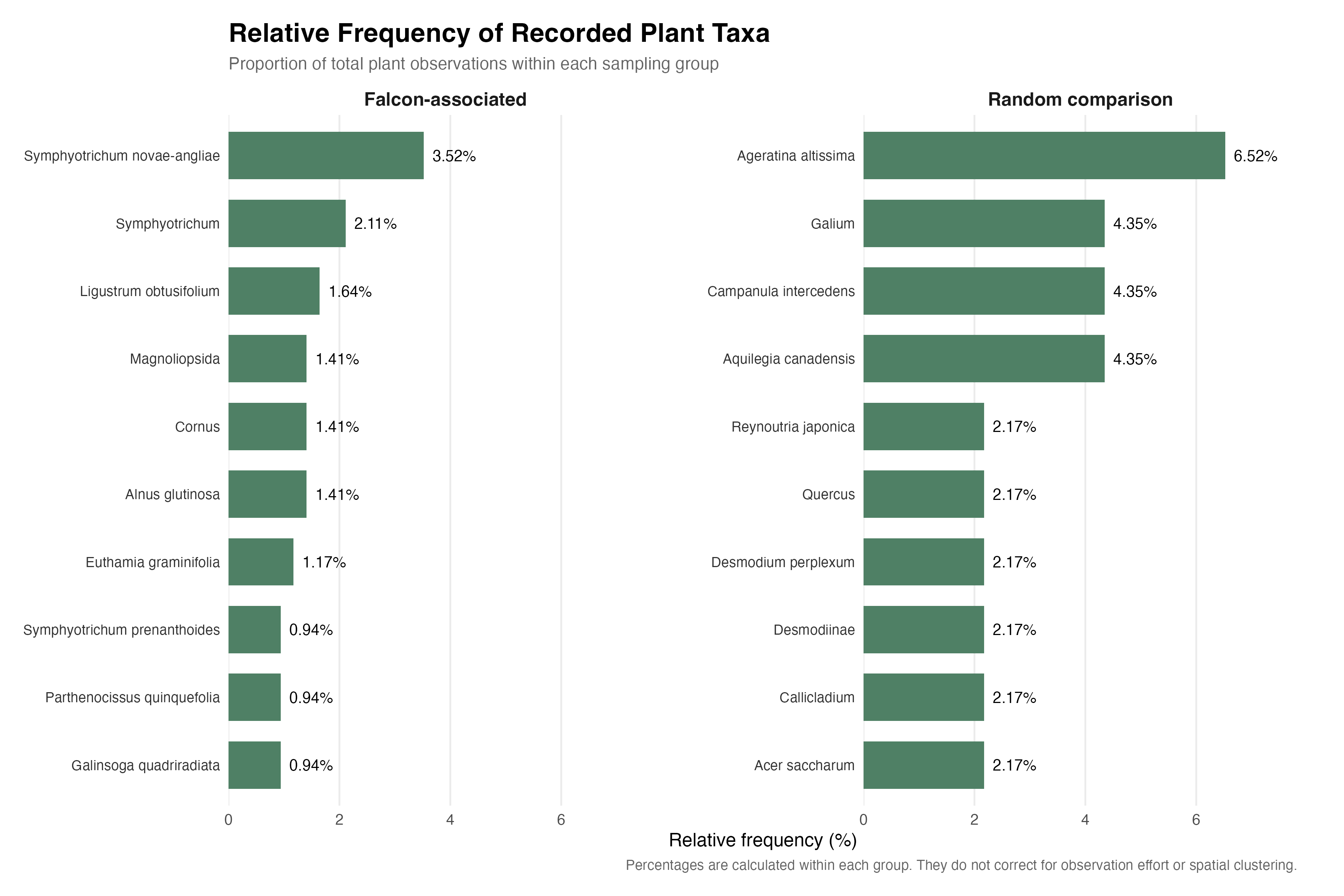
In the falcon-associated frequency table, the most frequent label was Symphyotrichum novae-angliae (15 records), followed by Symphyotrichum (9) and Ligustrum obtusifolium (7). In the random comparison table, Ageratina altissima was most frequent (3 records); Aquilegia canadensis, Campanula intercedens, and Galium each had 2 records. Labels may represent species, genera, or broader taxonomic groups, so they are not all equivalent species-level identifications.
The relative-frequency comparison provides a different view of the data. For example, Symphyotrichum novae-angliae accounts for 3.52% of falcon-associated plant records, while Ageratina altissima accounts for 6.52% of random-associated records. These percentages are calculated within each group and remain sensitive to observation effort and sample size.
Maps & figures
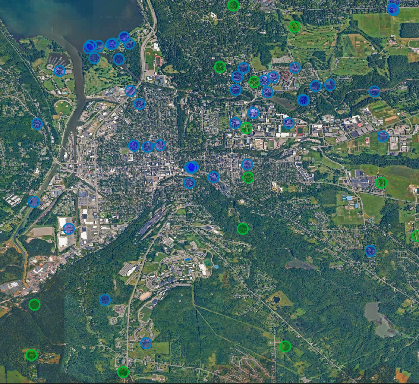
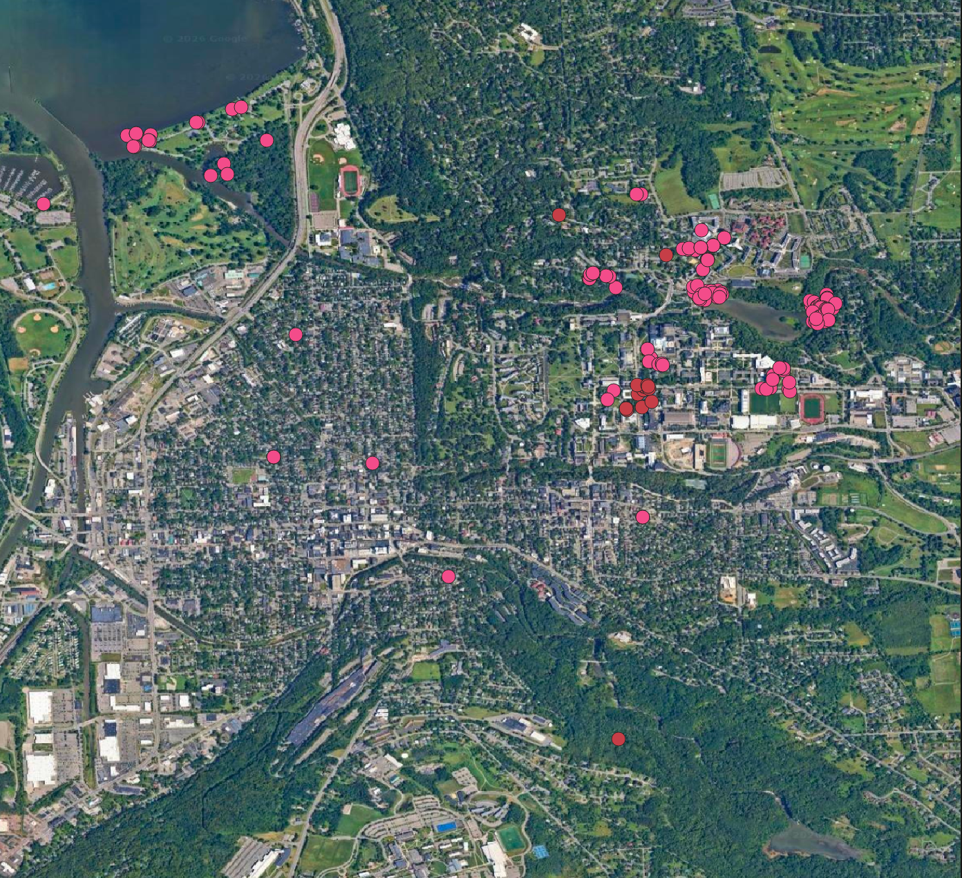
The eight figures document the study geography, sampling design, spatial distribution of plant records, taxonomic summaries, observation quality, and a key spatial limitation. Together, they show both the descriptive patterns and the design considerations that shape interpretation.
Data analysis in R
Descriptive analysis and figures completed · Inferential analysis not yet completedR was used to import the plant frequency tables, calculate within-group relative frequencies, identify the 18 shared taxonomic labels, summarize observation-quality composition, and produce the comparative charts shown above. These are descriptive analyses. No inferential test or model result is reported on this page.
Completed descriptive work
- Summarized raw taxonomic-label frequencies.
- Calculated within-group relative frequencies.
- Joined the frequency tables to identify exact shared labels.
- Compared iNaturalist observation-quality categories.
- Calculated intersecting buffer-pair counts.
Further analysis required
- Preserve unique observation IDs and distinguish observations from buffer associations.
- Build a complete buffer-level table, including buffers with zero plant records.
- Validate buffer geometry and distances in a projected CRS.
- Evaluate sampling effort, spatial dependence, seasonality, and taxonomic rank.
- Select and diagnose any inferential model only after the sampling structure is resolved.
Limitations & interpretation
Opportunistic observation data
iNaturalist records are contributed by users rather than collected through a standardized survey. Observer access, interests, activity, and timing can affect where records occur. Record counts are not direct measures of plant abundance.
Approximate buffer distance
The preliminary buffer operation used approximately 0.0009 degrees in EPSG:4326. This is not a uniform, exact 100-meter radius and should be treated as a limitation of the current spatial workflow.
Taxonomic resolution and observation quality
Some records are identified only to genus or broader taxonomic groups, and many are marked Needs ID. Taxonomic labels are not all equivalent to confirmed species identifications. Research Grade status is useful metadata but is not a guarantee of error-free identification.
These limitations do not make the project unusable. They define what can responsibly be concluded from the current data and provide a concrete roadmap for improving the sampling design and analysis.
Next steps
- Validate spatial methods: compare the existing angular buffers with buffers generated in a projected coordinate system using an exact distance in meters, then rerun the overlap and plant-selection operations.
- Audit repeated associations: use unique iNaturalist observation IDs to determine how often a plant record is associated with multiple buffers.
- Reconcile data tables: document how individual observations, buffer-observation associations, and summary counts relate to one another.
- Improve the comparison design: consider matching random locations by land cover, accessibility, season, and observation effort, and account for spatial clustering.
- Complete inferential analysis: conduct sensitivity analyses and select a defensible statistical approach only after the unit of analysis and sampling design have been validated.
- Document reproducibility: preserve data sources, API query parameters, access dates, QGIS processing steps, scripts, and analysis decisions.
The longer-term goal is to develop a repeatable approach for connecting community-contributed biodiversity records with spatial analysis. This project is an initial step toward using computational tools to support ecological research, conservation, and environmental decision-making.
References & data sources
https://doi.org/10.1093/jue/juab017
Relevant example of using public sighting records, GIS, and random comparison locations to investigate urban falcon habitat patterns. Its study design differs from this project.
https://doi.org/10.1093/biosci/biab093
Discusses spatial, temporal, and taxonomic biases in opportunistic iNaturalist observations.
https://www.inaturalist.org/
https://qgis.org/
Project data were collected from iNaturalist and processed for this exploratory analysis. Add the exact API query parameters, data access dates, and any applicable attribution to the project repository or a supplementary methods document for full reproducibility.